Introduction
Diffusion models play a major role in the recent success of AI systems that generate realistic images from natural language prompts; they lie at the core of OpenAI’s DALL·E 2, or Stability AI’s Stable Diffusion, for instance.
In this post we review the core ideas and walk you through the math to derive the loss function used to train those models. Mainly we follow the thoughts laid out in
“Denoising diffusion probabilistic models”, Jonathan Ho, Ajay Jain, and Pieter Abbeel, 2020.
However, we are bypassing the ELBO (Evidence Lower Bound) perspective and take a short cut that directly gets us to the simplified training loss (Eq. 14) and the reverse model in (Ho et al., 2020) – easing mathematical obfuscation. To us the approach presented here feels more intuitive than a detour through ELBO. We might lay out the more technically involved strategy in a different post, but for now we would like to add a perspective that the reader might not have seen already.
We hope that we can convince you that the core idea is relatively straightforward – depending on your background of course – and the actual challenge to make a system like DALL·E 2 work at scale seems to be one of engineering really.
Quick overview
- We start off by loosely defining the core intuition behind diffusion and how it could potentially be used to generate samples from a data distribution; cf. Section “The Core Idea”.
- We then define the forward diffusion process in detail; cf. section “The forward process”.
- Next, we pave our way to an approximation of its reverse; cf. section “The backwards process – Approximation of the reverse kernel”.
- Finally we explain how the simplified training loss fits in with the approximate reverse kernel; cf. Section “Simplifying the model to predict noise”.
The Core Idea
Loosely speaking — and paraphrasing Wikipedia here — diffusion is the process of something spreading out from a point of higher concentration into its lower concentrated surrounding. Usually this process goes along with an increase in entropy (informally the number of micro states in a macro arrangement), or a loss of “meaning”. Therefore, reversing the process would enable us to create something concrete out of something “meaningless”.
A bit more formally, in the context of (Ho et al., 2020) and this post, a diffusion process starts with an initial data distribution and defines a Markov chain with Gaussian transition kernels adding noise at each step along the chain. The kernels are chosen such that the further along in the chain we are the more the samples look normally distributed. Reversing this process we can generate new data samples by starting with Gaussian noise and inferring its origin.
 Figure 1: Exemplary roll outs of a $1$-dimensional diffusion process from left to right. The initial data distribution is shown on the left in magenta, and the distribution induced at the final stage of the process is shown on the right in blue.
The forward process
Let us put the above informal definition into symbols. Suppose we have a data set $X$ or even better a data distribution $Q_0$ we can sample from. A diffusion process is defined as a Markov chain with Gaussian transition kernels as follows: We first sample an initial data point $x_0$ from $Q_0$, then we successively add Gaussian noise and slowly push the data point towards the origin, to get samples $x_1, \ldots, x_T$, that is, for $t=1,\ldots,T$ we iteratively sample
\[x_t \ \sim \ Q(x_t \mid x_{t-1}) := N \big( x_t ; \mu_t(x_{t-1}), \Sigma_t \big),\]where
\[\mu_t(x_{t-1}) := \sqrt{\alpha_t} \cdot x_{t-1} \ \ \ \ \text{and} \ \ \ \ \Sigma_t := (1 - \alpha_t) \cdot I.\]The factors $\alpha_1, \ldots, \alpha_T$ are chosen such that at the final stage of the chain the $x_T$’s are approximately normal-distributed, i.e. we want our kernels to satisfy
\[Q(x_T \mid x_0 ) = \int_{x_1,\ldots,x_{T-1}} \prod_{t=1}^T Q(x_t \mid x_{t-1}) \ \ \text{d}x_0\cdots \text{d}x_{T-1} \stackrel{!}{\approx} \ N(0,I).\]Since all the kernels are Gaussian we can compute the distributions at all intermediate stages. With $\bar\alpha_t := \prod_{t’=1}^t \alpha_{t’}$ one can compute
\[\begin{eqnarray} Q_t(x_t \mid x_0 ) = N \big( x_t ; \sqrt{\bar\alpha_t}\cdot x_0 , (1 - \bar\alpha_t) \cdot I \big). \end{eqnarray}\]Thus the above condition for $Q(x_T \mid x_0 )$ to be approximately normal distributed translates to choosing $\alpha_1,\ldots,\alpha_T$ such that
\[\bar\alpha_T = \prod_{t=1}^T \alpha_{t} \stackrel{!}{\approx} 0 .\]The backwards process
As mentioned above we are bypassing the ELBO perspective and take a more direct path to derive the simplified training loss in (Ho et al., 2020). To us the approach presented here feels more intuitive than a detour through ELBO.
Approximation of the reverse kernel (without ELBO)
Now that we defined the forward process we can work our way towards reversing it. Our goal is to model the reverse kernel $Q(x_{t-1} \mid x_t)$. We choose our approximate model $P_\theta$ to be a diagonal Gaussian and set
\[P_\theta(x_{t-1} \mid x_t) = N \big( x_{t-1}; \mu_\theta(x_{t}), \sigma_t^2 \cdot I \big).\]We will only focus on mean $\mu_\theta(x_{t})$ of the model and ignore the parameters $\sigma_1, \ldots, \sigma_T$ for now.
The first thing one might try is to create training data by repeatedly sampling an initial point $x_0$ and rolling out the Markov chain to get samples $x_0, \ldots, x_T$. Then one could train the model to map $x_t$ to $x_{t-1}$. While this training recipe seems simple enough it is not very sample efficient. For $\mu_\theta(x_t)$ to converge to the true mean, $\mu^\ast$ say, we need quite a lot of sample paths that all pass through $x_t$. To tackle this efficiency problem we are going to identify a better target (cf. the definition of $\tilde\mu$ below) to update $\mu_\theta$ at each step in the training process; cf. Figure 2;
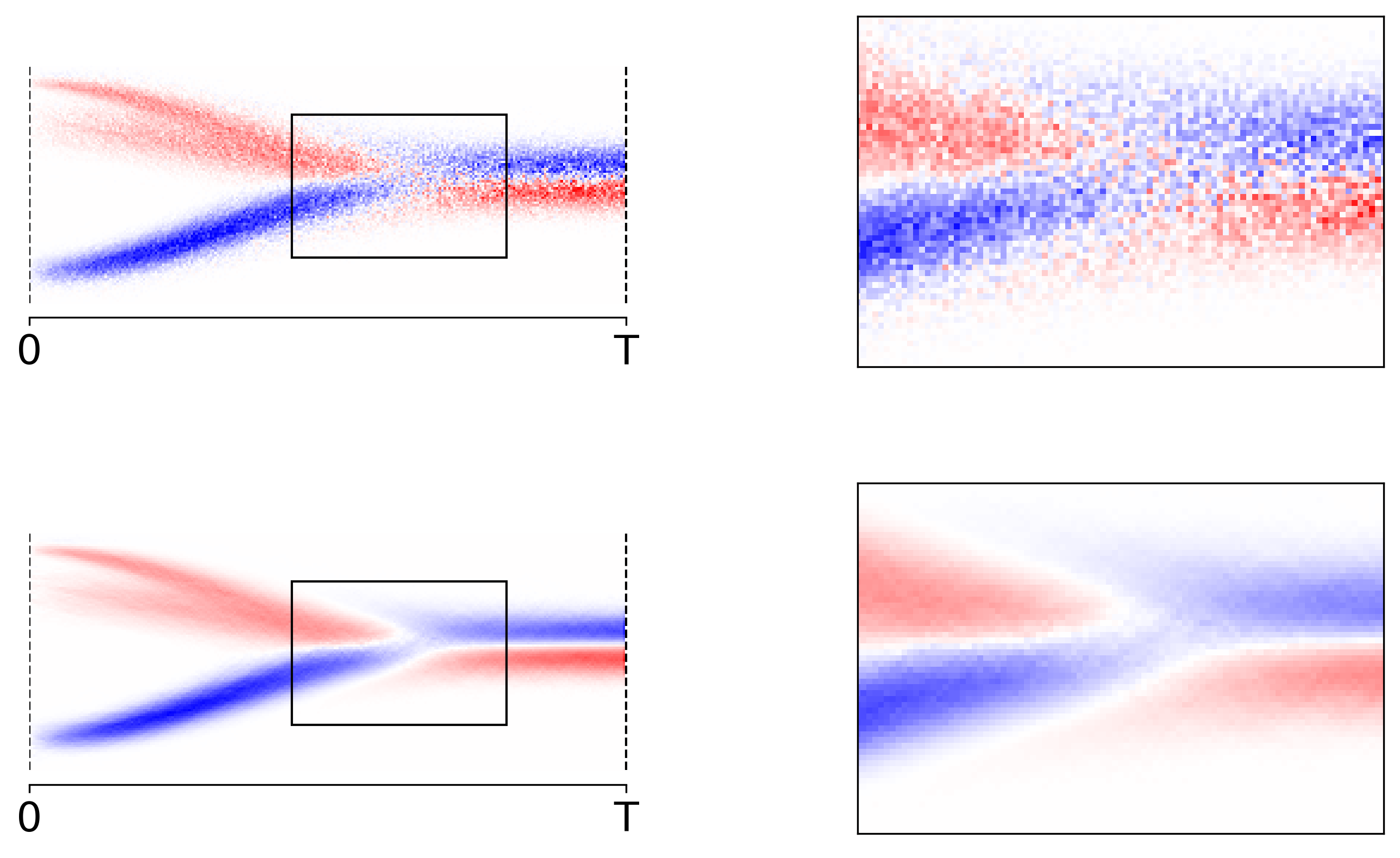 Figure 2: Note that in the $1$-dimensional we can visualize a reverse model, $\mu$ say, by coloring the pixels at $(t,x_t)$ by $\mu(x_t) - x_t$. In that light, the plot shows a 2D-histogram averaging $x_{t-1} - x_t$ (top) and $\tilde\mu(x_t) - x_t$ (bottom). Clearly, the latter approach converges much quicker than the naive sampling approach.
Here is what we would like to do: Instead of rolling out the whole chain we start with a sample $x_t$ from $Q(x_t)$, which we get by first sampling $x_0 \sim Q_0$ and then $x_t \sim Q(x_t \mid x_0)$. The desired target signal for the reverse mean model $\mu_\theta(x_t)$ would be given by the true mean $\mu^\ast(x_t)$ of the reverse model $Q(x_{t-1} \mid x_t)$, i.e. our objective would be to minimize something along the lines of
\[L^\ast := \mathbb{E}_{Q(x_t)} \Big[ \| \mu^\ast(x_t) - \mu_\theta(x_t) \|^2 \Big] .\]However, we don’t have access to $Q(x_{t-1} \mid x_t)$ in closed form. Applying Bayes’ rule doesn’t help us either since both $Q(x_{t-1})$ and $Q(x_t)$ have no obvious closed form. Fortunately we can rewrite $Q(x_{t-1} \mid x_t)$ as an expected value
\[\begin{eqnarray} Q(x_{t-1} \mid x_t) &=& \int_{x_0} Q(x_{t-1} , x_0 \mid x_t) \ \text{d}x_0 \\ &=& \int_{x_0} Q(x_{t-1} \mid x_0, x_t)\ Q(x_0 \mid x_t) \ \text{d}x_0. \end{eqnarray}\]We introduced the term $Q(x_{t-1} \mid x_0, x_t)$. Intuitively we might expect this term to be somewhat easier to figure out than $Q(x_{t-1} \mid x_t)$ since it carries information about the true initial state $x_0$. Applying Bayes’ rule and the Markov property of the chain one can show that the first term $Q(x_{t-1} \mid x_0, x_t)$ in the integral can be written as the product and quotient of three Gaussians and can in turn be expressed as a Gaussian itself. That means we can explicitly write down $\tilde\mu(x_t, x_0)$ and $\tilde\beta_t$ (see Eq. 7 in (Ho et al., 2020)) such that we have
\[\begin{eqnarray} Q(x_{t-1} \mid x_0, x_t) = N\big( x_t ; \tilde\mu(x_t, x_0), \tilde\beta_t\cdot I \big). \end{eqnarray}\]With this in hand we can use Eq. 3 to express the true target $\mu^\ast(x_t)$ as an expected value of accessible intermediate targets $\tilde\mu(x_t, x_0)$ (cf. Figure 3 below); we have
\[\begin{eqnarray} \mu^\ast(x_t) = \int_{x_0} \tilde\mu(x_t, x_0) \ Q(x_0 \mid x_t) \ \text{d}x_0. \end{eqnarray}\]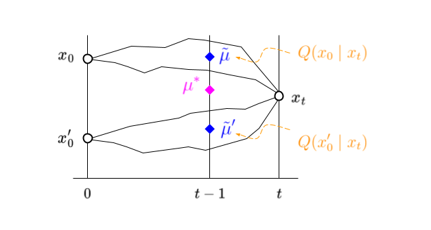
Figure 3: True target in magenta. Approximate target as a sum of partial targets in blue, weighted by their probability of occurrence in orange. The black lines indicate sample paths through $x_t$ starting at $x_0$ and $x_0’$ respectively.
Note that we can use $\tilde\mu(x_t, x_0)$ as a crude approximation for $\mu^\ast(x_t)$. Let us briefly go over why:
Technically, we sampled $x_0,x_t \sim Q(x_t, x_0) = Q(x_t \mid x_0)Q(x_0)$. Now suppose we got a trillion of those samples and suppose further $x_t$ takes only finitely many discrete values so we could bin the pairs with respect to a fixed $x_t$. Taking all pairs $(x^1_0,x_t), \ldots, (x^n_0,x_t)$ for a fixed $x_t$ we can approximate the integral by $\tfrac{1}{n}\sum_i \tilde\mu(x_t, x^i_0)$. In practice it is very (very) unlikely to hit some $x_t$ twice, so we find ourselves stuck with $n=1$ in the approximation. This is quite convenient, since we needed to sample $x_0 \sim Q_0$ first to be able to get a sample $x_t \sim Q(x_t \mid x_0)$ anyway.
From this viewpoint it makes somewhat sense that our objective becomes minimizing the distance between $\tilde\mu$ and $\mu_\theta$, or equivalently minimizing
\[\tilde{L} := \mathbb{E}_{Q(x_t \mid x_0)Q(x_0)} \Big[ \| \tilde\mu(x_t, x_0) - \mu_\theta(x_t) \|^2 \Big] .\]Simplifying the model to predict noise
The intuition behind the simplified training loss is simple: given $x_t$ predict $x_0$. We can then use the approximate reverse kernel from the previous section to sample $x_{t-1}$. All that is left to do to end up with the simplified loss in (Ho et al., 2020) is to rephrase the objective in terms of $x_0$, $t$, and $\epsilon$. Recall form Eq. 1 that $Q(x_t \mid x_0)$ is a diagonal Gaussian and we can generate samples by sampling $\epsilon \sim N(0,I)$ first and setting
\[\begin{eqnarray} x_t = \sqrt{\bar\alpha_t}\cdot x_0 + \sqrt{1- \bar\alpha_t}\cdot \epsilon. \end{eqnarray}\]That means we can express $x_t$ as a function of $x_0$, $t$, and $\epsilon$. Moreover, suppose we knew $\epsilon$, $t$, and $x_t$ then we can solve for $x_0$ and get
\[x_0 = \frac{1}{ \sqrt{\bar\alpha_t}}\big( x_t - \sqrt{1- \bar\alpha_t}\cdot \epsilon \big).\]This enables us to do two things: First, it means we can express our training target $\tilde\mu(x_t, x_0)$ as a function of $x_0$, $t$, and $\epsilon$. Our training target becomes
\[\tilde\mu(x_t, x_0) = \tilde\mu(x_0, t, \epsilon).\]Second, to model $\tilde\mu$ we only need to model the $\epsilon$ term, i.e. given a model $\epsilon_\theta(x_t,t)$ say, we could simply define
\[\mu_\theta(x_t, t) := \tilde\mu(x_0, t, \epsilon_\theta(x_t, t)).\]Note that we never explicitly wrote down $\tilde\mu$ anywhere, since we do not really need to in order to get to the training objective. However, if we wanted to actually run the reverse model to generate new data samples we need the expression for $\tilde\mu$ which can be found in (Ho et al., 2020) (Eq. 7). Fitting $\epsilon_\theta(x_t,t)$ yields our final objective (cf. Eq. 14 in (Ho et al., 2020))
\[\begin{eqnarray} L_\text{simple} = \mathbb{E}_{x_0,t,\epsilon} \Big[ \big\| \epsilon - \epsilon_\theta\big( x_t(x_0, t, \epsilon),t \big) \big\|^2 \Big]. \end{eqnarray}\]References
- Ho, J., Jain, A., & Abbeel, P. (2020). Denoising Diffusion Probabilistic Models. ArXiv Preprint Arxiv:2006.11239.