Ordering points to identify the clustering structure (OPTICS) is a data clustering algorithm presented by Mihael Ankerst, Markus M. Breunig, Hans-Peter Kriegel and Jörg Sander in 1999 (Kriegel et al., 2011). It builds on the ideas of DBSCAN (Ester et al., 1996), which I described in a previous post. But let’s cut the intro and dive right into it.

Idea

Let $(X,d)$ be a finite discrete metric space, i.e. let $X$ be a data set on which we have a notion of similarity expressed in terms of a suitable distance function $d$. Given a positive integer $m \in \mathbb{N}$ we can define a notion of density on points of our data set, which in turn can be used to define a perturbed metric. Given a starting point $x_0 \in X$ the OPTICS-algorithm iteratively defines a linear ordering on $X$ in terms of a filtration $X_0 \subset X_1 \subset \ldots \subset X_n$ of $X$, where $X_{n+1}$ is obtained from $X_n$ by appending the closest element (with respect to the perturbed metric) in its complement.

The original OPTICS-algorithm also takes an additional parameter $\varepsilon > 0$. However this is only needed to reduce the time complexity and is ignored in our discussion for now – to be more precise, we implicitly set $\varepsilon = \infty$.

Definitions

Let $(X,d)$ be a finite discrete metric space and $m \in \mathbb{N}$ a positive integer. We define the (co-)density $\delta_m(x)$ of a point $x$ by

\[\delta_m(x) := d(x, \mathfrak{nn}_m(x)),\]

where $\mathfrak{nn}_m(x) $ is an $m$-nearest-neighbor of $x$. Loosely speaking: the lower the value $\delta_m(x)$ the closer the neighbors of $x$ are distributed around $x$. Note that with $\varepsilon = \delta_m(x)$ the point $x$ is a core point in the sense of (Ester et al., 1996) – in a previous post about DBSCAN we called such a point $\varepsilon$-dense. That is why in the literature $\delta_m(x)$ is referred to as core-distance. I however like to think of it, and hence refer to it, as a notion of co-density. Given the co-density $\delta_m(.)$ we can define the reachability distance $r_x(y)$ of $y$ from $x$ by

\[r_x(y) := \text{max} \big\{ \delta_m(x), d(x,y) \big\}.\]

Note that $r_x(y)$ is not symmetric, since the density of $x$ and $y$ may differ.

Sketch of the algorithm

Choose a starting point $x_0 \in X$. Then we can iteratively define a filtration $X_0 \subset \ldots \subset X_n$ of the data set $X$ by

\[X_0 := \{ x_0 \} \ \ \text{and} \ \ X_{k+1} := X_k \cup \{ x_{k+1} \},\]

where $x_{k+1}$ minimizes $r_{X_k}(.)$ over $X \setminus X_k$. In parallel we define a sequence $(r_n)$ of distances by

\[r_0 = 0 \ \ \text{and} \ \ r_{k+1} := r_{X_k}(x_{k+1}).\]

Note that a small distance $r_k$ may be understood as $x_k$ being close to a rather dense region. Therefore the filtration tries to stay in dense regions for as long as possible, before it passes a less dense region. The cluster structure can now be extracted by analyzing the reachability-plot, that is a $2$-dimensional plot, with the ordered $x_k$ on the $x$-axis and the associated distances $r_k$ on the $y$-axis. By the above considerations it should be clear that clusters show up as valleys in the reachability plot. The deeper the valley, the denser the cluster.

Example

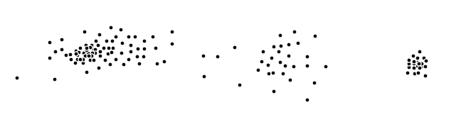
Consider the data points $X\subset \mathbb{R}^2$ in the euclidian plane given in the following figure:

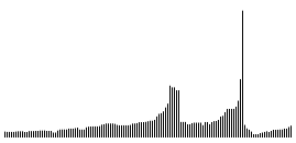
Below you see the reachability plot corresponding the OPTICS-algorithm applied to the above data set with $m=4$. The starting point is chosen among the group of points on the left.

References

1. Kriegel, H.-P., Kröger, P., Sander, J., & Zimek, A. (2011). Density-based clustering. WIREs Data Mining and Knowledge Discovery , 1(3), 231–240. https://doi.org/https://doi.org/10.1002/widm.30
2. Ester, M., Kriegel, H.-P., Sander, J., & Xu, X. (1996). A Density-Based Algorithm for Discovering Clusters in Large Spatial Databases with Noise. Proceedings of the Second International Conference on Knowledge Discovery and Data Mining, 226–231.