Quite a while ago I stumbled over a white paper (Numenta, 2011) of a science startup called Numenta. At the core of the paper lies the model of a sequence memory that enables the prediction of elements in a time series based on its history of predecessors. An essential ingredient in the model are sparse distributed representations, a binary data structure motivated by recent findings in neuroscience, where it was observed that sparse activation patterns are used by the brain to process information (e.g. in early auditory and visual areas).

The goal of this post is (a) to briefly recall what sparse representations are, and (b) how to encode real-world data as sparse representations. We roughly follow Numenta’s approach and connect it to a construction well-known in computational topology called witness complex – a simplicial complex that can be understood as a simplicial approximation of the inputs space.

Sparse distributed representations

The space of patterns

Let $X$ denote a discrete set of $n$ elements. Think of it as an (a priori unordered) collection of bits, \(\{1,\ldots, n\}\) say. Denote by $\mathcal{P} =\mathcal{P}_n$ the power set of $X$, i.e.

\[\mathcal{P} := \big\{ p : p \subset X \big\}.\]

We will refer to elements in $\mathcal{P}$ as patterns. An intuitive example would be to think of $X$ as representing a family of pixels, and a pattern representing the collection of black pixels of a black-and-white image. There are two natural operations on $\mathcal{P}$, namely the union of sets $\cup$, and the intersection of sets $\cap$. The latter in fact gives rise to a notion of similarity of two patterns $p$ and $p’$ in terms of their intersection or overlap. We define the overlap count of $p,p’$ as

\[\omega(p,p') := |p\cap p'|.\]

Intuitively: the bigger the overlap the more similar the two patterns are. This is a somewhat vague notion – since we do not incorporate the individual sizes of the patterns – but for now we do not want to bother too much about that, when we restrict our attention to sparse patterns, in the respective section below, this notion of similarity becomes more accurate.

Patterns as binary vectors

Note that we can naturally identify the power set of $n$ elements $\mathcal{P}$ with \(\{0,1\}^n\), the boolean algebra of $2^n$ elements, as follows: recall that $\mathcal{P}$ denotes the power set of a set of $n$ distinct elements, \(\{ 1,\ldots,n \}\) say. Then one easily checks that the desired isomorphism from \(\{0,1\}^n\) into $\mathcal{P}$ is given by

\[(v_1,\ldots,v_n) \mapsto \{ i : v_i=1 \}.\]

With respect to the above identification the union of sets $\cup$ corresponds to the componentwise or-operation $\vee$ on \(\{0,1\}^n\), and the intersection of sets $\cap$ corresponds to the componentwise and-operation $\wedge$ on \(\{0,1\}^n\). Therefore we indeed have

\[\big(\mathcal{P};\cup,\cap \big) \cong \big(\{0,1\}^n ; \vee, \wedge \big).\]

Note that we could understand \(\{0,1\}^n\) as embedded into $n$-dimensional Euclidean Space $\mathbb{R}^n$. Then the above notion of similarity corresponds to the euclidean scalar product of two vectors. This viewpoint allows us to pull back any distance, or scalarproduct, defined on $\mathbb{R}^n$ to $\mathcal{P}$. We can pull back the metric induced by the $L^1$-norm on $\mathbb{R}^n$, for instance, which yields the the Hamming distance on \(\{0,1\}^n\) (interpreted as binary strings). We may come back to that later.

Sparse patterns and their natural metric

The central objects in (Numenta, 2011) are sparse representations. For some fixed positive integer $k \ll n$ we call a pattern \(p \in \mathcal{P}\) sparse if the number of elements in $p$ satisfies \(\vert p \vert = k\). Finally we denote by $SDR = SDR(k,n)$ the set of sparse patterns in $\mathcal{P}$ and refer to its elements as sparse (distributed) representations, i.e. we define

\[SDR := \big\{ p \in\mathcal{P} : |p| = k \big\}.\]

The terminology presumes (and only makes sense in combination with) a sparse encoder satisfying certain properties. We describe a particular construction of such an encoder below. It is easy to check that the notion of similarity $\omega$, defined above, gives rise to an honest metric $d = d_k$ on the subset of sparse patterns $SDR$ defined by

\[d_H(p,q) := k - |p \cap q|.\]

This is equivalent to the Hamming distance (up to a constant factor of $2$) on \(\mathcal{P}\) restricted to the set of sparse patterns.Let us also define a softer version of sparse representations by including patterns with less or equal than $k$ elements, i.e. we define

\[SDR_{\leq k} := \big\{ p \in\mathcal{P} : |p| \leq k \big\}.\]

REMARK. (Sparseness after Olshausen and Field) In (Olshausen & Field, 1997) sparseness turned up within a probabilistic framework where the authors try to match the probability distribution over images observed in nature by a generative linear model. However, in contrast to our approach, the coefficients in (Olshausen & Field, 1997) are allowed to take values in $\mathbb{R}$. The notion of sparseness then corresponds to assuming a certain prior probability distribution over the coefficients, whose density is shaped to be unimodal and peaked at zero with heavy tails, implying that coefficients are mostly inactive. However there is no restriction on the actual number of active units. If we would like to emphasize this difference, we will refer to a sparse vector in the sense presented here as a binary sparse vector. However it should always be clear from the context what definition is referred to.

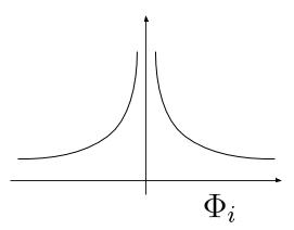Fig. Probability density of sparse coefficients in the sense of Olshausen and Field

Spatial pooling and weak witness complexes

In the present section I introduce a geometrical perspective on how to encode inputs sampled from a metric space as sparse representations. We follow an idea analogous to the approach in (Numenta, 2011) and connect it to a construction well-known in computational topology called witness complex (see (Silva & Carlsson, 2004) and cf. also (Carlsson, 2009)).

Let $(X,d)$ be a, not necessaryly discrete, metric space, e.g. $X = \mathbb{R}^m$ endowed with the Euclidean distance. Our goal is the construction of a map

\[\Phi \colon\thinspace X \to SDR \subset \mathcal{P}_n.\]

We refer to such a map $\Phi$ as an (untrained) spatial pooler or (binary) sparse encoder. In another post we address different notions of what it means for an encoder to be trained on a collection of inputs $Y \subset X$. Let me first describe a way to construct such a map. Choose a family of $n$ landmarks

\[L=\{ l_1,\ldots,l_n\} \subset X.\]

These landmarks can be understood as features, or elements of a codebook (an overcomplete basis of the input space). Given an input $x \in X$ we assign to it the collection of indices $\Lambda (x) \subset {1,\ldots,n}$ of the $k$ closest landmarks, i.e. we define

\[\Lambda (x) := \Lambda^{(k)}_L(x) := \{ i_1, \ldots , i_k \},\]

such that $d(x, l_{i}) < d(x, L \setminus { l_{i_1},\ldots,l_{i_k} } )$ for each $i \in \Lambda (x)$. Here $d(x,Y)$ deotes the the minimal distance of a point $x$ to the elements in a finite set $Y$. Note that in general this assignment is not well-defined since the set of $k$ closest landmarks may not be unique – in practice however this can always be achieved by adding a tiny random perturbation to each landmark, or by fixing a rule of precedence, e.g. prefer the landmark with the lower index. (The latter approach for instance is taken in the spatial pooler implementation of Numenta’s open source library NuPIC up to version 0.3.5; the latter up from version 0.3.5. – update: I recently was told that the random perturbation was fixed so it was the latter version all along)

REMARK. (Landmarks in Numenta’s Spatial Pooling)  We can interpret the permanence values of the synaptic connections of a particular column in (Numenta, 2011) as a landmark.

For each $i \in \Lambda (x)$ we call $x$ a weak witness (or for simplicitly just witness) for $l_i$ – note that our definition of a witness slightly differs from the construction in (Carlsson, 2009), but it still captures the essence of the construction. (We also give a slight variation of this notion below)

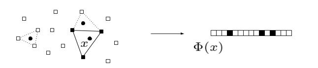Fig. Three points in $X$ on the left and the sparse representation $\Phi(x)$ of one of them as a binary vector (shown on the right). The vertices of the dotted triangles indicate the representations of the other two remaining points (not shown on the right). The squares represent the landmarks.

For a lack of better imagination we refer to the collection of witnesses

\[W(l) := \{ x : \text{$x$ is a witness for $l$} \}.\]

associated to a particular landmark $l$ as its associated (depth-$k$) witness cell. Note that for $k=1$ the witness cell of a landmark equals its associated Voronoi cell. We could also be interested in the the collection of common witnesses associated to a family of landmarks $l_{i_1},…, l_{i_q}$ and hence define

\[W( l_{i_1},..., l_{i_q} ) := \bigcap_{i \in } W(l_i).\]

This obviously generalizes the above notion of a depth depth-$k$ witness cell, and therefore we stay with the terminology. Analogous to the simpler version, for $k=q$ this equals the order-$q$ Voronoi region associated to $l_{i_1}, …, l_{i_q}$. Below we describe how we can use these notions to define a simplicial complex associated to a collection of inputs. Obviously we can understand $\Lambda(x)$ as an element of $SDR({k,n})$ for each $x \in X$, and hence the assignment

\[\Phi \colon\thinspace x \mapsto \Lambda (x)\]

defines the desired map. To train an encoder on a collection of inputs translates into the right choice of landmarks. I will address that in another post.

Witnesses with respect to similarity

Suppose, instead of an honest metric we are given a notion of similarity on \(X\) expressed in terms of a non-negative function

\[\omega \colon\thinspace X \times X \to \mathbb{R}_{\geq 0}.\]

Consider the $m$-dimensional cube \([0,1]^m\) endowed with the Euclidean dot product, for instance. Then the above construction of $\Lambda$ also follows through if we look for the $k$ most similar landmarks – instead of the $k$ closest landmarks. To be more precise we define \(\Lambda (x) := \{ i_1, \ldots , i_k \}\) such that \(\omega(x, l_{i}) < \omega(x, l_j)\) for each $i \in \Lambda (x)$ and $j \not\in \Lambda (x)$.

Restricting the sight of witnesses

Instead of assigning the $k$ closest (or most similar respectively) landmarks to a point, we can further restrict the set the potential landmarks to be within a certain radius, $\theta < 0$ say. To be more precise, $x$ is a witness with sight $\theta$ for $l$ iff $l$ is among the $k$ closest landmarks and $x$ is contained in the ball of radius $\theta$ centered at $l$, i.e. $d(x,l) < \theta$. The problem with this approach is that we have to ensure that we find $k$ landmarks to form a complete sparse representation, i.e. one that has exactly $k$ active bits. This can be achieved e.g. by adding random elements to the representation until completion, or by fixing a rule of precedence upon which we choose elements to complete the representation.

A way around this is to establish a softer version of sparse representations, e.g. allow patterns with less or equal than $k$ elements. (This is effectively what was going on in Numenta’s open source implementation NuPIC up to version 0.3.5: if there are less than $k$ landmarks within sight of $x$, i.e. with distance $d(x,l) < \theta$, the non-complete representation is randomly extended to a complete one – update: apparently the random choice is fixed once at the beginning) This then yields a variation of the above sparse encoder with values in $SDR_{\leq k}$ defined by

\[\Lambda_\theta(x) := \big\{ l : d(x,l) < \theta \text{ and $l$ is among the $k$ closest landmarks} \big\}.\]

Approximation by simplicial complexes

Suppose we are given a collection of inputs $Y \subset X$. Then there is a simplicial complex $\mathcal{W}(Y,L)$, the (weak) witness complex (cf. (Carlsson, 2009; Silva & Carlsson, 2004)), whose vertex set is given by $L$, and where \(\Lambda = \{l_{i_1},..., l_{i_q}\}\) spans a $q$-simplex iff there is a common witness for all landmarks in $\Lambda$, i.e. if $W(l_{i_1},…, l_{i_q}) \neq \emptyset$. An obvious variation of this complex is obtained by restricting the set of witnesses to those with sight $\theta$. We denote this complex by $\mathcal{W}_\theta(Y,L)$. This obviously defines a subcomplex of the (weak) witness complex. Usually we are interested in the subcomplexes of dimension less or equal than $k$, and we can understand the witness complexes as an simplicial approximation of the data $Y \subset X$.

References

1. Numenta. (2011). Hierarchical Temporal Memory (HTM) Whitepaper. https://numenta.com/neuroscience-research/research-publications/papers/hierarchical-temporal-memory-white-paper/
2. Olshausen, B. A., & Field, D. J. (1997). Sparse coding with an overcomplete basis set: A strategy employed by V1? Vision Research, 37(23), 3311–3325. https://doi.org/https://doi.org/10.1016/S0042-6989(97)00169-7
3. Silva, V. de, & Carlsson, G. (2004). Topological estimation using witness complexes. In M. Gross, H. Pfister, M. Alexa, & S. Rusinkiewicz (Eds.), SPBG’04 Symposium on Point - Based Graphics 2004. The Eurographics Association. https://doi.org/10.2312/SPBG/SPBG04/157-166
4. Carlsson, G. (2009). Topology and Data. Bull. Amer. Math. Soc., 46, 255–308.